-

Background

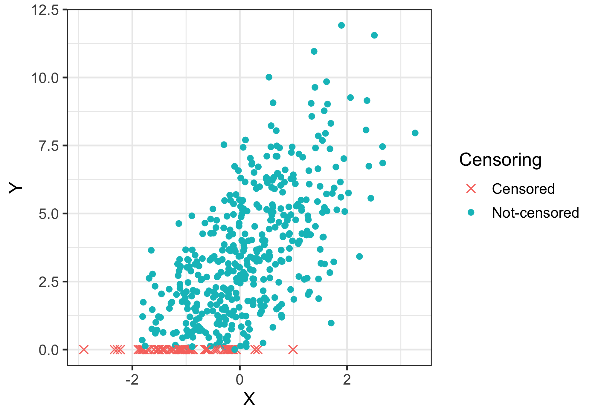
We recently got an interesting request from our collaborators from the bench side. They have two types of experimental assays, let’s call them assay X and assay Y, that measure the activity of the same biological pathway. The difference between them is that assay Y has a limit of detection of certain value U, and it reports any value lower than U as U; on the contrary, X is much sensitive and effectively have no limit of detection. In other word, Y is left-censored, whereas X is not censored at all. A simulated data is shown below.

Our collaborators would like to learn how “consistent” these two assays are. A popular metrics for between-assay consistency is Pearson correlation coefficient. However, it is obviously inappropriate to be used here, unless the censoring is accounted for. In addition, we need not only the point estimation, but also a confidence interval, of correlation coefficient. To address this challenge, one of my colleagues developed an approach to robustly estimate Pearson correlation coefficient (and its credible interval) for such censored data. The original workflow was implemented in JAGS and SAS. I am curious if I can recreate the analysis using R and Stan (I mean, why not?). So here we go!

Simulate a toy example data

Let \(X\) be a random variable, and define random variable \(Y\) as:

…and \(Y\) is left-censored at a known threshold, 0:

An example of simulated toy data is shown as below:

Stan model

We then define the following model using Stan. It imputes censored data points of \(Y\), and Pearson correlation coefficient is computed as:

data {
  int<lower=0> N_obs;          // Number of observed data points
  int<lower=0> N_cens;         // Number of censored data points
  vector[N_obs] x_obs;      // Observed predictor matrix
  vector[N_cens] x_cens;    // Censored predictor matrix
  vector[N_obs] y_obs;
  real sd_x;
}

transformed data{
  int<lower=0> N;
  N = N_obs + N_cens;
  
  vector[N] x;
  x = append_row(x_obs, x_cens);
  
  
}

parameters {
  real beta;       // coefficients for predictors
  real alpha;
  real<lower=0> sigma;  // error scale
  vector<upper=0>[N_cens] y_cens;
}

transformed parameters {
  
  vector[N] y_imputed;
  y_imputed = append_row(y_obs, y_cens);
  
  real cov_x_y;
  cov_x_y = sum((y_imputed - mean(y_imputed)) .* (x - mean(x))) / (N-1);
  
  real<lower=0> sd_y;
  sd_y = sqrt(square(beta * sd_x) + square(sigma));
  
  real<lower = -1, upper=1> rho;
  rho = cov_x_y/sd_x/sd_y;
  
}
model {
  y_obs ~ normal(alpha + x_obs * beta, sigma);  // target density - observed points
  y_cens ~ normal(alpha + x_cens * beta, sigma); // target density - censored points
}

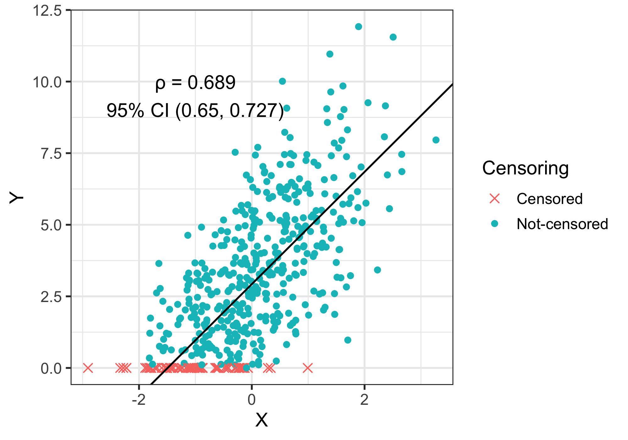
Since \(\rho\) is computed for each draw, we can then obtain the posterior distribution of \(\rho\) and get its 95% credible interval. And here is the final output, where the simulated data, the point estimation and 95% credible interval of \(\rho\), and a regression line of \(X\) and \(Y_{imputed}\) are shown on the same plot:

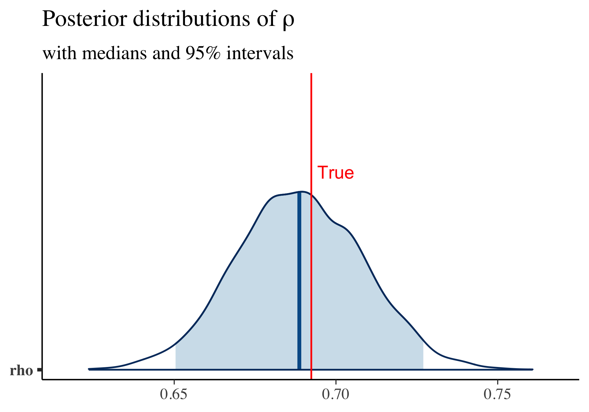
And the posterior distribution of \(\rho\) and the ground-truth value of \(\rho\) are shown below:

Recap

• Several R packages allow one to fit censored data using Tobit model. One advantages of using Bayesian analysis, instead, is the ability of analyzing complex model,e.g. hierarchical models.