-

Background

Droplet-based single-cell RNA sequencing (scRNA-seq) data are often considered to be zero-inflated, meaning they contain zero counts in many cells, even for the gene that are supposed to be expressed in all of them. These excess zeros are typically attributed to both biological factors (stochastically bimodal pattern of RNA expression) and technical artifacts (like dropout events due to molecular inefficiencies).

However, a recent study challenged this assumption by analyzing negative control scRNA-seq datasets, data generated by measuring pre-made RNA samples that shall not exhibit any biological variability in gene expression. Surprisingly, the authors found that these data are not zero-inflated. Instead, the observed count distributions were well explained by a negative binomial (NB) distribution, suggesting that much of the observed sparsity may be inherent to the count-generating process itself.

In this post, I explore the implications of this finding by modeling droplet-based, UMI-tagged scRNA-seq data using the negative binomial distribution.

Model specification

The model I use is based on the negative binomial framework described in the DESeq2 paper, with some modifications to suit the characteristics of single-cell RNA-seq data.

Let \(K_{ij}\) represents read count for gene \(i\) in sample \(j\), and we model these counts as:

Here:

• \(\mu_{ij}\) is the mean of the distribution of read count,
• \(\phi_i\) is the shape parameter controls the overdispersion.

The \(\mu_{ij}\) is further modeled as:

where:

• \(\rho_{ij}\) is the true expression level of gene \(i\) in sample \(j\),
• \(s_j\) is the sequencing depth of sample \(j\), a.k.a size factor of sample \(j\).

Key Difference from DESeq2

One key difference between this model and DESeq2’s model lies in how shape parameter \(\phi\) is estimated. DEseq2 is typically used for bulk RNA-seq dataset with relative small sample size, and accurate estimation of both mean and shape parameter from such limited data can be challenging or even impossible. Thus, DEseq2 assumes genes of similar average expression strength have similar dispersion, and this allows sharing information across genes. However, single cell data usually have much larger sample size (here each individual cell can be regarded as a sample), so that we can accurately estimate both \(\phi\) and \(\mu\) directly.

Dataset

The data used in this analysis come from Zheng et al., a negative control dataset generated by sequencing ERCC synthetic spike-in RNAs using the 10X Genomics platform. The dataset includes measurements for 92 RNA species across 1,015 droplets, with no expected biological variation, making it ideal for evaluating statistical properties of count distributions.

Stan model

The negative binomial model described above was implemented in Stan:

• Each gene is modeled independently and we estimate \(\mu_{ij}\) and \(\phi_i\) for one gene at a time.
• Careful choice of priors significantly improves computational efficiency. See recommendations from Stan team.
• Use profile() function in Stan code to access the computational cost of different parts of the model.

On my personal laptop, fitting each gene takes approximately 10 seconds.

data {
  int<lower=0> N; // number of cells
  vector[N] total_count_per_cell;
  array[N] int y; // read count of the gene in cells
}

parameters {
  real log_q;
  real<lower=0> reciprocal_sqrt_phi; 
}

transformed parameters {
  vector[N] log_mu;
  real phi;
  
  profile("mat_multi"){
    log_mu = rep_vector(log_q, N) + log(total_count_per_cell);
    phi = 1/square(reciprocal_sqrt_phi);
  }

}

model {
  profile("likelihood"){
    log_q ~ normal(0, 10);
    reciprocal_sqrt_phi ~ normal(0, 10);
    y ~ neg_binomial_2_log(log_mu, phi);
  }
  
}

Model Checking

We can evaluate a Bayesian model specification and its fit to the data in many ways. As described in this paper, common approaches include:

• Prior predictive check helps diagnose priors that are not appropriate to the data - too strong, too weak, poorly shaped, or poorly located.
• Model fitting using varieties of diagnostic statistics and plots.
• Posterior predictive check helps to examine whether a model does a good job of capturing relevant aspects of the data.

Posterior predictive simulation is implemented using following Stan code:

generated quantities {
  array[N] int y_sim;
  
  for (n in 1:N) {
    y_sim[n] = neg_binomial_2_rng(exp(log_mu[n]), phi);
  }

}

Here, we show 8 draws from posterior predictive distribution and compare it to the empirical data:

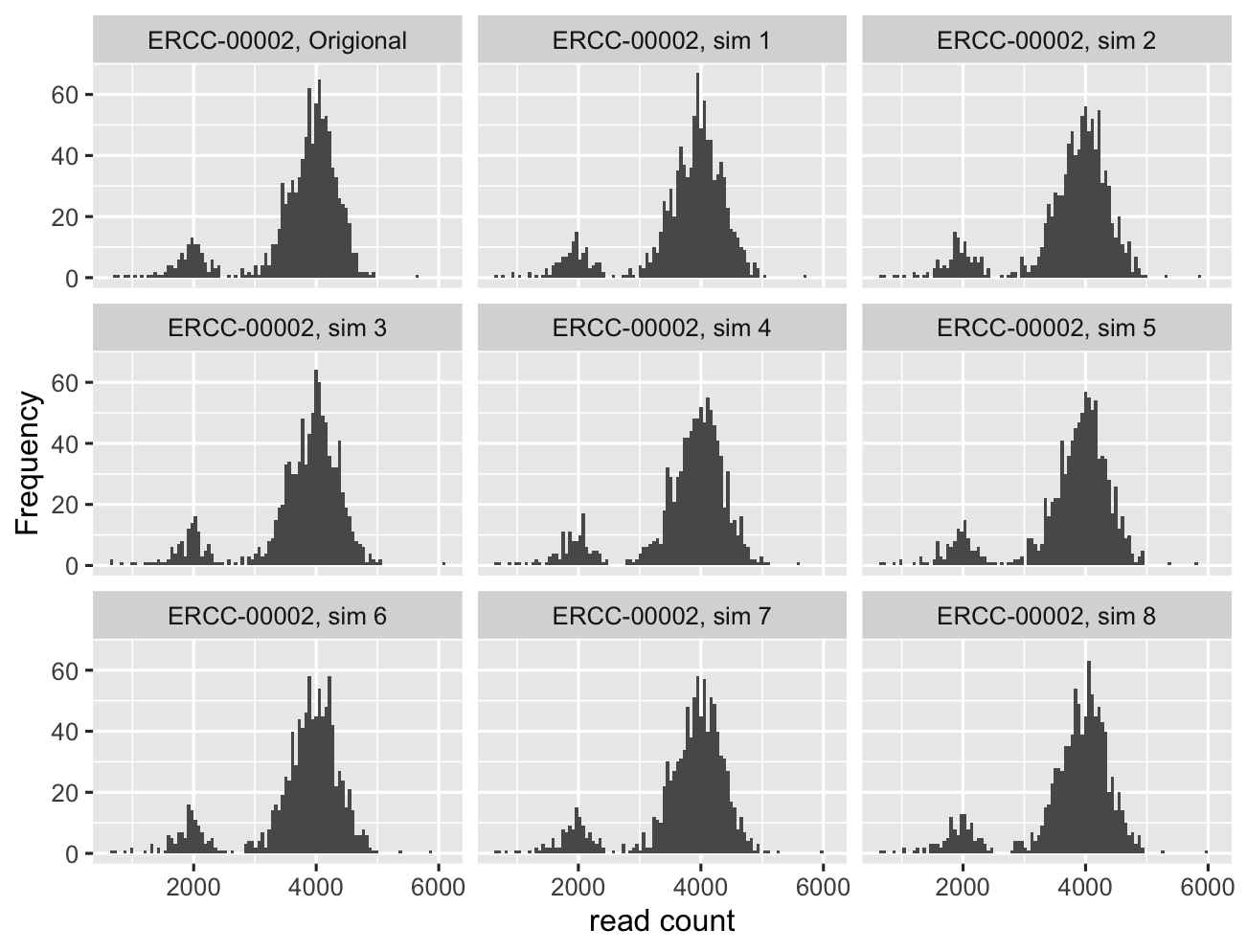
… we see data simulated from posterior distribution resembles the real data very well.

Result validation

As a validation, I exam the relationship between estimated ERCC RNA concentrations and their known molecular concentration provided by the manufacturer. As shown in the plot below, the two are in strong agreement, suggesting that \(q\) serves as a reliable estimate of true RNA abundance.

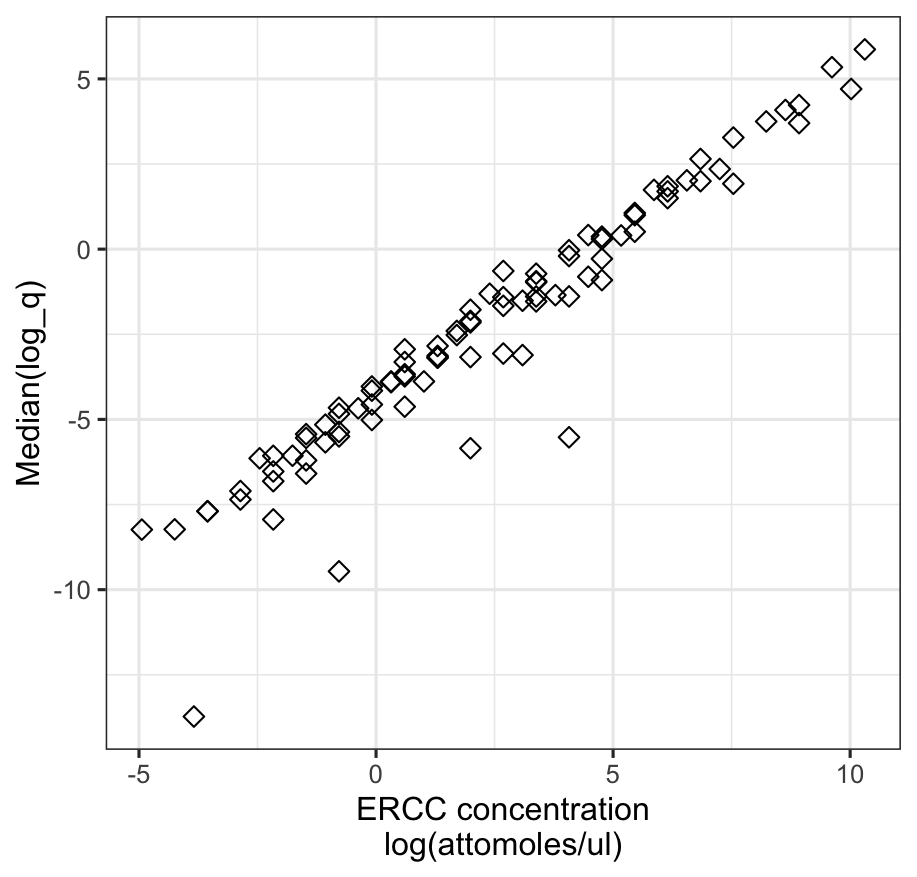
However, a few RNA species appear to be underestimated, with their inferred concentrations falling noticeably below the overall linear trend (e.g., the four outlier points in the plot). This suggests that some transcripts may be less efficiently captured or sequenced in practice.

I plan to look into the causes of this discrepancy in more detail in a future post 🙂