Using posterior predictive likelihood to access cell quality in scRNA-seq
Published:
-
Background
The posterior predictive likelihood of a data point quantifies how well that point is explained by a Bayesian model. Formally, the posterior predictive distribution is given by:
\[\displaylines{ p(\tilde{x}|X_{train}) = \int_{\theta} p(\tilde{x}|\theta)p(\theta|X_{train})d\theta }\]Suppose we fit a Bayesian model using a training dataset \(X_{train}\), and then evaluate the posterior predictive likelihood of a new data point \(\tilde{x}\). This likelihood tends to be higher when \(\tilde{x}\) is similar to the training data and lower when it deviates from the learned patterns.
In the context of single-cell RNA-seq data, this framework can be applied to ERCC spike-in transcripts to assess data quality for individual droplets. These spike-ins have known concentrations that are expected to remain constant across droplets, assuming good droplet quality. Thus, a Bayesian model trained on ERCC counts from high-quality droplets should assign high posterior predictive likelihood to ERCC counts in other high-quality droplets.
Conversely, if a droplet is of poor quality, its ERCC read count apttern may deviate significantly from the expected distribution, resulting in a lower posterior predictive likelihood. This provides a principled way to identify and filter out low-quality cells in downstream analysis.
Model implementation
We first implement a Bayesian as below.
- Parameters declared in block “model” will not be saved in fit$draws.
functions {
  vector repeat_vector(vector input, int K) {
    int N = rows(input);
    vector[N*K] repvec; // stack N-vector K times

    for (k in 1:K) {
      for (i in 1:N) {
        repvec[i+(k-1)*N] = input[i]; // assign i-th value of input to i+(k-1)*N -th value of repvec
      }
    }
    return repvec;
  }

vector rep_each(vector x, int K) {
    int N = rows(x);
    vector[N * K] y;
    int pos = 1;
    for (n in 1:N) {
      for (k in 1:K) {
        y[pos] = x[n];
        pos += 1;
      }
    }
    return y;
  }

}

data {
  int<lower=0> N; // total number of data point. n_gene * n_cell
  int<lower=0> n_gene;
  int<lower=0> n_cell;
  vector[N] total_count_per_cell;
  vector[n_gene] x;
  array[N] int y;
}

parameters {
  vector<lower=0>[n_gene] reciprocal_sqrt_phi;
  real alpha;
  real beta;
  real<lower=0> sigma;
  vector[n_gene] log_q;
}

transformed parameters {
    vector[N] log_mu; // N = n_gene * n_cell
    vector[N] phi;
    log_mu = repeat_vector(log_q, n_cell) +
            log(total_count_per_cell);
    phi = repeat_vector(1/square(reciprocal_sqrt_phi), n_cell);

}

model {

  alpha ~ normal(0,10);
  beta ~ normal(-10,10);
  sigma ~ normal(0, 10);
  reciprocal_sqrt_phi ~ normal(0, 10);
  log_q ~ normal(alpha + beta * x, sigma);
  y ~ neg_binomial_2_log(log_mu, phi);

}
Compute log-likelihood of testing dataset
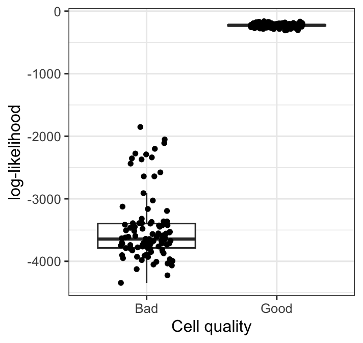
We simulate bad-quality cells by shuffling read count values of 10 randomly picked ERCC transcripts.
We then compute their point-wise log-likelihood for each cell in the testing data, which contains 400 good cells and 100 bad cells. Likelihood computation is done with cmdstanr’s standalone generated quantities method, using Stan code as below:
functions {
  vector repeat_vector(vector input, int K) {
    int N = rows(input);
    vector[N*K] repvec; // stack N-vector K times

    for (k in 1:K) {
      for (i in 1:N) {
        repvec[i+(k-1)*N] = input[i]; // assign i-th value of input to i+(k-1)*N -th value of repvec
      }
    }
    return repvec;
  }

vector rep_each(vector x, int K) {
    int N = rows(x);
    vector[N * K] y;
    int pos = 1;
    for (n in 1:N) {
      for (k in 1:K) {
        y[pos] = x[n];
        pos += 1;
      }
    }
    return y;
  }
}

data {
  int<lower=0> N; // total number of data point. n_gene * n_cell
  int<lower=0> n_gene;
  int<lower=0> n_cell;
  vector[N] total_count_per_cell;
  vector[n_gene] x;
  array[N] int y;
}

parameters {
  vector<lower=0>[n_gene] reciprocal_sqrt_phi;
  real alpha;
  real beta;
  real<lower=0> sigma;
  vector[n_gene] log_q;
}

transformed parameters {
    vector[N] log_mu; // N = n_gene * n_cell
    vector[N] phi;
    log_mu = repeat_vector(log_q, n_cell) +
            log(total_count_per_cell);

    phi = repeat_vector(1/square(reciprocal_sqrt_phi), n_cell);

}

generated quantities {
  vector[n_cell] log_lik;
  real log_q_log_lik;

  log_q_log_lik = normal_lpdf(log_q | alpha + beta * x, sigma);

  for (n in 1:n_cell) {
    log_lik[n] = neg_binomial_2_log_lpmf(y[((n-1)*n_gene+1):n*n_gene] |
                  log_mu[((n-1)*n_gene+1):n*n_gene],
                  phi[((n-1)*n_gene+1):n*n_gene]) + log_q_log_lik;
  }
}
We see a very distinct difference between log-likelihood of good cells vs bad cells.