-

Background

The Expectation-Maximization (EM) algorithm is a powerful method for estimating parameters in statistical models that include unobserved or latent variables. In such models, the log-likelihood depends on the latent variables, and the marginal log-likelihood \(l(\theta)\) (which integrates over the latent variables) often lacks an analytical solution, making direct maximization intractable.

The EM algorithm provides a practical, iterative approach to approximate the maximum likelihood estimates (MLE) of the parameters of interest. Many excellent resources explain the EM algorithm in depth. For instance, this blog post derives the general form of the EM algorithm and explains why it converges to a local maximum. This video offers a more intuitive demonstration of how the EM algorithm works, and this tutorial implements EM for estimating parameters in a Gaussian mixture model, but only for one parameter \(\pi\).

Rather than repeating the theory behind the EM algorithm, this post will focus on a hands-on implementation: using the EM algorithm to estimate the MLE of \(\theta = (\mu_1, \mu_2, \pi_1)\) in a bimodal Gaussian mixture model.

Data simulation

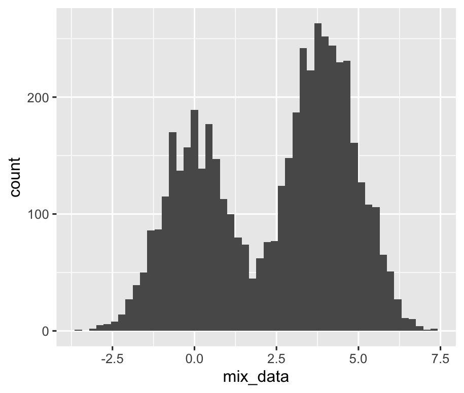
We first simulate a toy dataset where \(X \sim GauMix(\mu_1, \mu_2, \pi_1)\), where sd of both Gaussian components are known and equal to 1.

pi_s = 0.4; u1_s = 0; u2_s = 4

mix_data = sapply(runif(5000), FUN = function(x){
  
  if(x<pi_s){
    return(rnorm(n = 1, mean = u1_s))
  }else{
    return(rnorm(n = 1, mean = u2_s))
  }
  
})

The histogram of mix_data are shown below:

Implementing EM algorithm for bimodal Gaussian mixture model in R

We implemented the EM algorithm in R to compute the maximum likelihood estimate (MLE) for \(\theta = (\mu_1, \mu_2, \pi_1)\) in a bimodal Gaussian mixture model.

For simplicity, we used only one set of initial values for \(\theta\). The algorithm stops when converges (delta log likelihood < 1e-5) or after 50 iterations, whichever comes first.

######################
# implement EM algorithm

calc_resp = function(xi, u1, u2, pi_1, pi_2){
  w_k1 = pi_1 * dnorm(xi, u1)
  w_k2 = pi_2 * dnorm(xi, u2)
  
  resp_k1 = w_k1 / sum(w_k1, w_k2)
  resp_k2 = w_k2 / sum(w_k1, w_k2)
  #browser()
  return(c(resp_k1, resp_k2))
}


EM.iter <-function(mix_data, u1, u2, pi_1){
  resp_k1_list = c()
  resp_k2_list = c()
  
  for(xi in mix_data){
    temp = calc_resp(xi, u1, u2, pi_1, 1 - pi_1)
    resp_k1_list = c(resp_k1_list, temp[1])
    resp_k2_list = c(resp_k2_list, temp[2])
  }
  
  N_k1 = sum(resp_k1_list)
  N_k2 = sum(resp_k2_list)
  
  pi_1_new = N_k1 / length(mix_data)
  
  u1_new = sum(resp_k1_list * mix_data) / N_k1
  
  u2_new = sum(resp_k2_list * mix_data) / N_k2
  
  return(c(u1_new, u2_new, pi_1_new))
}


calc.log.lik <- function(mix_data, u1, u2, pi_1, pi_2){
  log.lik.list = c()
  for(xi in mix_data){
    temp = log(pi_1 * dnorm(xi, u1, sd = 1) + pi_2 * dnorm(xi, u2, sd = 1))
    log.lik.list = c(log.lik.list, temp)
  }
  return(sum(log.lik.list))
}

#######################

# initialization:
u1_curr = -3; u2_curr = 3; p1_curr = 0.3; 
log.lik = -Inf

# save intermediate results:
u1_list = c()
u2_list = c()
p1_list = c()
p2_list = c()

for(i in c(1:50)){
  
  log.lik_curr = calc.log.lik(mix_data, u1_curr, u2_curr, p1_curr, 1 - p1_curr)
  
  if(log.lik_curr - log.lik < 1e-5){
    break
  }else{
    log.lik = log.lik_curr
  }
  
  temp = EM.iter(mix_data, u1_curr, u2_curr, p1_curr)
  
  u1_curr = temp[1]; u2_curr = temp[2]; p1_curr = temp[3]; 
  
  u1_list = c(u1_list, u1_curr)
  u2_list = c(u2_list, u2_curr)
  p1_list = c(p1_list, p1_curr)
  p2_list = c(p2_list, 1 - p1_curr)
  
}

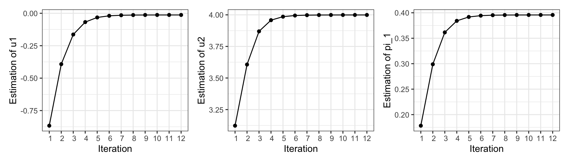
The algorithm converged after 12 iterations. The plots below illustrate how the estimated values of each parameter evolved over the course of the iterations.