-

Background

I encountered the following question at work: I have a response variable pf interest that is censored at both ends, that is, subjected to both left- and right- censoring, and I want to model its relationship with several covariates. I decided to use a hierarchical Bayesian linear regression model.

Let \(Y_i\) denote the measurement outcome of sample \(i\). Following the concept of Bayesian modeling, the data generating process can be described as below:

where \(Y_i\) is the true (latent) response variable, and \(Y_{\text{lower-limit}}\) and \(Y_{\text{upper-limit}}\) are fixed constants representing the lower and upper limits of detection of the assay. When the true measurement falls outside the detectable range, the instrument reports the corresponding detection limit rather than the true value.

While implementing this model using the R package brms, I noticed some apparent inconsistencies in how such data censoring should be specified. In particular, a discussion on brms Github page suggests to model such response variable as a Interval-censored data. And this seems contradictory to descriptions found elsewhere, such as here and Kruschke et. al. p732. These resources suggest that interval censoring refers to observations for which the true value lies within a specified interval are censored, while values outside that interval are observed directly. I therefore decided to look into this in more details by running some simulations, to make sure I use brms in the right way.

Simulations

###########################
rm(list=ls())
library(brms)
library(tidyverse)
library(ggplot2)
library(patchwork)

###########################
# simulation parameters
set.seed(1993)
options(mc.cores = 4)

n = 500
a = 10
b=5
sigma = 3

##########################
# simulate example data
df = data.frame(x = rnorm(n = n)) %>% # predictor x
  mutate(y = a + b*x + rnorm(n = n, sd = sigma)) %>% # outcome y
  mutate(y_cen = case_when(y <= 5 ~ 5,
                           y >= 20 ~ 20,
                           .default = y)) %>% # add censoring
  mutate(censored = case_when(y <= 5 ~ "left",
                              y >= 20 ~ "right",
                              .default = "none"))

##########################
# fit model using brms
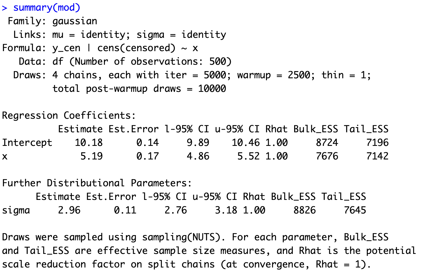
mod <- brm(y_cen | cens(censored) ~ x,
            data = df, iter = 5000)

summary(mod)

##########################
# check against ground truth
p1 = df %>% pivot_longer(cols = c(y, y_cen)) %>% 
  ggplot(aes(x = value)) +
  geom_histogram(color = "white", 
                 fill = "skyblue4", linewidth = 0.25) +
  facet_wrap(~ name, ncol = 1, scales = "free_y")+
  labs(x = NULL,
       subtitle = "Data")

p2 = predict(mod,
              summary = FALSE,
              ndraws = 4) %>%  
  data.frame() %>%  
  mutate(sim = 1:n()) %>% 
  pivot_longer(cols = -sim) %>% 
  ggplot(aes(x = value)) +
  geom_histogram(color = "white", 
                 fill = "skyblue", linewidth = 0.25) +
  geom_vline(xintercept = 5, linetype = 2) +
  geom_vline(xintercept = 20, linetype = 2) +
  labs(x = NULL,
       subtitle = "Simulations") +
  facet_wrap(~ sim, labeller = label_both, ncol = 2)

# plot
p1 + p2 + 
  plot_layout(widths = c(1, 2)) +
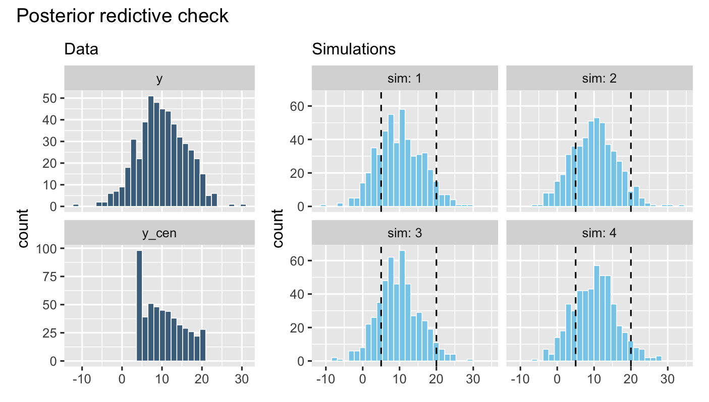
  plot_annotation(title = "Posterior predictive check")

We then compare the model estimates with the ground truth. As we can see, the 95% creditable intervals of \(a\) and \(b\) both contain the true parameter values:

In addition, posterior predictive checks show that the fitted model can generate new data whose distribution closely resembles that of the observed data: